Table of Contents
- I. What is Net-Trim?
- II. Net-Trim Code: Step By Step Demo
- III. Net-Trim Code: More Technical Demo
- IV. Net-Trim Versions
- V. How to Cite Net-Trim?
I. What is Net-Trim?
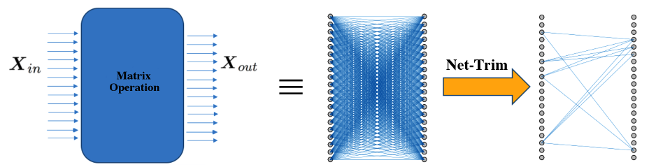
A (deep) neural network can be considered as a cascade combination of processing blocks, where each block is composed of a linear operator (representable by a matrix), and a nonlinear unit. Each block matrix may contain thousands and millions of parameters, which are hard to store, interpret and operate through. Net-Trim is a post-processing module, which applies to a network that is already trained (any sophisticated technique used for the initial training is fine with Net-Trim), and simplifies the network architecture by pruning each block. Net-Trim reprocesses the network block by block, in way that the response of each block to the input data remains almost intact and similar to the initial model, while the input/output relation is stablished via a much simpler operation.
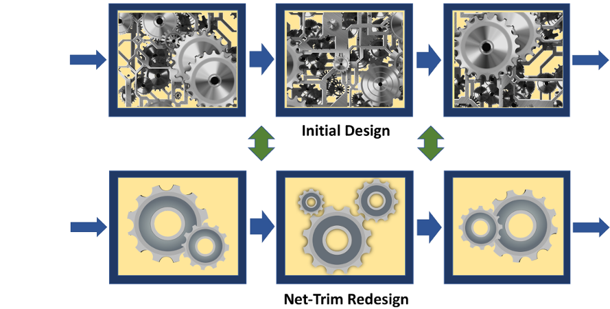
The pruning of each layer is performed by solving a convex optimization problem, which sets a large portion of the matrix entries of each block to zero. In a sense, Net-Trim disconnects many redundant connections of the network by directing the processing load to a small portion of the connections. Net-Trim shares many technicalities with LASSO for linear models and can be considered as a way of applying LASSO to (deep) neural networks.
In networks with ReLU activation, the input and output of each layer are related via
where is the input data matrix with each column corresponding to a training sample, is the learned weight matrix and is the output data matrix. Net-Trim basically finds a (sparse) matrix to replace , via a convex variant of the following program:
I.1. Why Using Net-Trim to Simplify Neural Networks?
One of the long-standing problems with the neural networks is their excessive parameterization, which makes them hard to interpret, and prone to overfitting. While augmenting the model complexity is capable of reducing the training error (reducing the bias), it can hurt the model predictability and cause an accuracy loss for the test data. Net-Trim pruning can be beneficial from various standpoints:
- Faster predictions, by making the network matrices sparse
- Memory/storage efficiency, by significantly reducing the number of network parameters
- Improving the test accuracy by removing network redundancies and simplifying the architecture (similar to the LASSO)
- Making the models more interpretable and even identify important input/intermediate features
I.2. What is Special About Net-Trim and Its Convex Formulation?
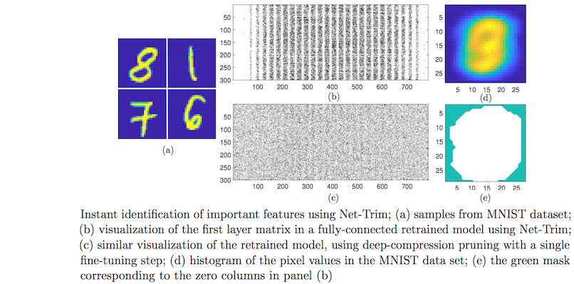
Net-Trim core process is framed as a convex program, which makes it insensitive to local optimality and initialization. Basically, running Net-Trim on a fixed network always produces the same result. Not only a convex formulation is desirable from a computational standpoint, it also allows a performance analysis of Net-Trim from a mathematical perspective. Comparatively speaking, heuristic methods such as deep compression present no convergence guarantees and require several thresholding operations followed by fine tuning steps to prune a network. Net-Trim operates much faster, since a fine tuning step is only an optional step for it, and even if exploited, a single, one-time fine tuning step is sufficient. The following figure compares the ability of Net-Trim and deep compression to extract important input pixels.
Also, compared to more recent techniques such as L-OBS (layer-wise optimal brain surgeon) Net-Trim is orders of magnitude faster (Net-Trim retraining of the LeNet network on a desktop computer only takes few minutes, while inverse-Hessian calculations for L-OBS requires hours/days of processing).
I.3. Additional Readings and Multimedia
For more technical details about the Net-Trim formulation and the way it works we invite you to consult the following papers:
- NIPS, 2017: “Net-Trim: Convex Pruning of Deep Neural Networks with Performance Guarantee”
- Journal Paper, 2020: “Fast Convex Pruning of Deep Neural Networks”
or the video presentations:
II. Net-Trim Code: Step By Step Demo
In this section we go through a pedagogical and step by step application of the Net-Trim, including the initial training, the pruning and the optional fine tuning. For this section, all you need is the NetTrimSolver_tf.py code from the Main NetTrim Solvers folder. For a more advanced but efficient implementation using a wrapper function, please refer to the next section.
In the sequel we train a convolutional neural network (CNN), prune it and apply a fine tuning step. Simply, use the following Python code to build a CNN model on the MNIST dataset:
# A CNN model for the MNIST Dataset
import numpy as np
import copy
import time
import NetTrimSolver_tf as nt_tf
import ConvNetTrimSolver_tf as cnt_tf
import keras
from keras.datasets import mnist
from keras.models import Sequential
from keras.layers import Dense
from keras.layers import Dropout
from keras.layers import Flatten
from keras.layers.convolutional import Conv2D
from keras.layers.convolutional import MaxPooling2D
from keras.utils import np_utils
from keras.backend import set_image_dim_ordering

strides = [1, 1, 1, 1]
padding = 'SAME'
data_folder = 'SomePath/'

# defining model
def my_model():
    # create model
    _model = Sequential()
    _model.add(Conv2D(20, (5, 5), input_shape=(1, 28, 28), activation='relu', strides=strides[1:-1], padding=padding))
    _model.add(MaxPooling2D(pool_size=(2, 2)))
    _model.add(Conv2D(10, (3, 3), activation='relu', strides=strides[1:-1], padding=padding))
    _model.add(MaxPooling2D(pool_size=(2, 2)))
    _model.add(Dropout(0.2))
    _model.add(Flatten())
    _model.add(Dense(128, activation='relu'))
    _model.add(Dense(50, activation='relu'))
    _model.add(Dense(num_classes, activation='softmax'))
    # compile model : setting the training algorithm
    _model.compile(loss='categorical_crossentropy', optimizer='adam', metrics=['accuracy'])
    return _model
We now start training the model. For a faster training we only use 5 epochs, you can increase it to as many as you would find necessary:
set_image_dim_ordering('th')
seed = 7
np.random.seed(seed)
# load data
(X_train, y_train), (X_test, y_test) = mnist.load_data()

# reshape to be [samples][pixels][width][height]
X_train = X_train.reshape(X_train.shape[0], 1, 28, 28).astype('float32')
X_test = X_test.reshape(X_test.shape[0], 1, 28, 28).astype('float32')

# normalize inputs from 0-255 to 0-1
X_train = X_train / 255
X_test = X_test / 255

# one hot encode outputs
y_train = np_utils.to_categorical(y_train)
y_test = np_utils.to_categorical(y_test)
num_classes = y_test.shape[1]
# define the larger model

# build the model
model = my_model()
# # In case you have already saved a model
# model.load_weights(data_folder + 'trained_weights.h5')
# Fit the model: For more accurate results increase epochs to 10 or more
model.fit(X_train, y_train, validation_data=(X_test, y_test), epochs=1, batch_size=200)
# In case you want to save the trained model
model.save_weights(data_folder + 'trained_weights.h5')
Let’s assess the model accuracy:
# Initial evaluation of the model
scores = model.evaluate(X_test, y_test, verbose=0)
print("Accuracy of the Initially Trained Model: %.2f%%" % (scores[1] * 100))
At this point, we have a trained network. We can extract the coefficient matrices, along with the input/output data associated with each layer.
# inputs and outputs of the layers of the trained model
org_weights = model.get_weights()

inputs = [layer.output for layer in model.layers]
layer_inputs = keras.backend.function([model.input, keras.backend.learning_phase()], inputs)

# using a subset of the training data for Net-Trim retraining (use 55000 to apply full data)
data_subset_size = 20000
data_index = np.random.choice(np.arange(X_train.shape[0]), data_subset_size, replace=False)

X = layer_inputs([X_train[data_index, :, :, :], 0])
X = [X_train[data_index, :, :, :]] + X

# In case, you want to save signals and weights
np.savez_compressed(data_folder + 'nn_data.npz', *X)
np.savez_compressed(data_folder + 'nn_org_weights.npz', *org_weights)
For now, let’s only extract the matrices corresponding to the fully connected (FC) layers (layers 3, 4 and 5) and the corresponding signals of the layers. Note that when applying Net-Trim we do not necessarily need to use the entire training data and even a subset of the data would suffice. For instance here we can use 20K samples instead of the full 55K ones. Let’s now apply the Net-Trim stand-alone code to each layer to acquire a new sparse weight matrix. You would only need , and choose a value of to retrain a layer (see the second program in Section IV). The value that you pass as is relative, for instance if you set , the actual that the program uses is . We apply Net-Trim to layers 2, 3 and 4 as reflected in the loop below. Here we used for all the layers. The parameter rho is the ADMM penalty parameter that depends on the data scaling, here yields a reasonably fast convergence. The number of ADMM iterations are controlled by the product of unroll_number and max_iterations, where the former is the number of loops performed within the GPU and the latter indicates the exterior loops. Overall, the total ADMM iterations are the product of the two and normally 300 to 500 totall iterations are enough for a proper convergence. For the last layer that usually no activation is used, Net-Trim program reduces to a sparse least-squares program.
# Net-Trim pruning for the fully connected layers
# indices of the signals input to the fully connected layers, and the corresponding weights and biases
fc_layers = [6, 7, 8]
fc_w_index = [4, 6, 8]
fc_b_index = [5, 7, 9]

unroll_number = 10
max_iterations = 40
# defining a Net-Trim class for the fully connected layers
nt_fc = nt_tf.NetTrimSolver(unroll_number=unroll_number)

epsilon_gain = 0.05
nt_weights = copy.deepcopy(org_weights)

for k in range(3):
    x = np.concatenate([X[fc_layers[k]].transpose(), np.ones((1, data_subset_size))])
    y = X[fc_layers[k] + 1].transpose()

    if k < 2:
        # ReLU layer, use net-trim
        V = np.zeros(y.shape)
    else:
        # use sparse least-squares (for the last layer, ignore the activation function)
        wh = np.concatenate([org_weights[fc_w_index[k]], org_weights[fc_b_index[k]][np.newaxis, :]])
        y = np.matmul(wh.transpose(), x)
        V = None

    norm_Y = np.linalg.norm(y)
    epsilon = epsilon_gain * norm_Y

    start = time.time()
    # main Net-Trim call
    W_nt = nt_fc.run(x, y, V, epsilon, rho=1, num_iterations=max_iterations)
    elapsed = time.time() - start

    # store the trimmed parameters
    nt_weights[fc_w_index[k]] = W_nt[:-1, :]
    nt_weights[fc_b_index[k]] = W_nt[-1, :]

    print('elapsed time = ', elapsed)
II.1. Retraining the Convolutional Layers
Since the convolution operator is a linear operator, Net-Trim formulation conveniently extends to such layers. The only additional component is dealing with tensors instead of matrices. While the convolution operator and the data tensors can be converted to matrices and vectors to apply the standard Net-Trim formulation, one can directly work with operators and avoid such conversion. We suggest consulting the following document which explains the details of applying Net-Trim when the linear operator is not in a matrix form. This implementation only requires forming the adjoint operator and replaces the Net-Trim least squares solve with a series of conjugate gradient iterations:
The retraining of the convolutional layers can become faster if the conjugate gradient iterations become stochastic. The following code prunes the convolutional layers (it however does not use the stochastic version of the conjugate gradient).
# Net-Trim pruning for the convolutional layers
# indices of the signals input to the convolutional layers, and the corresponding weights and biases
conv_layers = [0, 2]
conv_w_index = [0, 2]
conv_b_index = [1, 3]

unroll_number = 1
max_iterations = 400
# defining a Net-Trim class
nt_conv = cnt_tf.NetTrimSolver(unroll_number=unroll_number, cg_iter=10, strides=strides, padding=padding, precision=32)

epsilon_gain = 0.05
for k in range(2):
    x = X[conv_layers[k]]
    y = X[conv_layers[k] + 1]
    W = org_weights[conv_w_index[k]]
    b = org_weights[conv_b_index[k]]

    # transform data into the correct format, BxHxWxD (b/c of the Keras defaults, not necessary in general)
    x = np.transpose(x, axes=(0, 2, 3, 1))
    y = np.transpose(y, axes=(0, 2, 3, 1))

    V = np.zeros(y.shape)

    norm_Y = np.linalg.norm(y)
    epsilon = epsilon_gain * norm_Y

    start = time.time()
    # main Net-Trim call
    W_nt = nt_conv.run(x, y, V, b, W.shape, epsilon, rho=1, num_iterations=max_iterations)
    elapsed = time.time() - start

    nt_weights[conv_w_index[k]] = W_nt
    nt_weights[conv_b_index[k]] = b

    print('elapsed time = ', elapsed)

# save model's parameters
np.savez_compressed(data_folder + 'trimmed_weights.npz', *nt_weights)
Let’s build a new model with the retrained sparse weights and compare the accuracy and the number of nonzeros of the initial and the retrained models matrices:
# evaluation of the original model
model.set_weights(org_weights)
org_scores = model.evaluate(X_test, y_test, verbose=0)

# evaluation of the trimmed model
model.set_weights(nt_weights)
nt_scores = model.evaluate(X_test, y_test, verbose=0)

# number of non-zero coefficients
str_nnz = ', '.join('{}'.format(np.count_nonzero(np.abs(w) > 1e-4)) for w in org_weights[4::2])
print("Original CNN model: accuracy = {0:.3f}, number of non-zeros = {1}".format(org_scores[1], str_nnz))

# number of non-zero coefficients
str_nnz = ', '.join('{}'.format(np.count_nonzero(np.abs(w) > 1e-4)) for w in nt_weights[::2])
print("Pruned CNN model : accuracy = {0:.3f}, number of non-zeros = {1}".format(nt_scores[1], str_nnz))
The value of is a trade-off between the model sparsity and bias (training accuracy). Sometimes, when you use large ’s in the Net-Trim program to gain more sparsity, the network loses some accuracy. Often times a fine tuning round, where the network is trained again only updating the nonzero entries and initialized from the Net-Trim output can further improve the accuracy. This step-by-step demo was only a very quick and naiive way of implementing the Net-Trim. In Section III we explain how to use a wrapper that conveniently builds the initial model, applies Net-Trim and performs a round of fine tuning to further improve the results.
III. Net-Trim Code: More Technical Demo
In this section we go through a more advanced application of Net-Trim, which makes use of easy-to-use wrapper functions and includes a fine-tuning step. Having a GPU can speed up the process. Right now the Lenet retraining is done in about 3 minutes. To run this section, only the material provided in the Wrapper Example folder is needed. The wrapper functions allow building a model, training it, apply Net-Trim and finally fine-tune the Net-Trim output. The code below (also available as NetTrimWrapper.py) performs all these steps:
import time
import numpy as np
import copy
from tensorflow.examples.tutorials.mnist import input_data
from BasicLenet import BasicLenetModel
from PrunedLenet import PrunedLenetModel
import NetTrimSolver_tf as nt_tf
import os
os.environ['TF_CPP_MIN_LOG_LEVEL'] = '2'
mnist = input_data.read_data_sets('MNIST_data', one_hot=True)

# list of parameters to tune:
# training batch size
batch_size = 200
# training Dropout probability
keep_prob = 0.75
# training max number of iterations
mx_iter = 2001

# Net-Trim parameters:
# number of loops inside GPU
unroll_number = 10
# number of loops outside the GPU
num_iterations = 30
# relative value of epsilon for Net-Trim
epsilon_gain = 0.15

# create neural network and train
nn = BasicLenetModel()
nn.create_network()
nn.create_optimizer(training_algorithm='Adam', learning_rate=0.001, decay_rate=0.98, decay_step=500)
nn.create_initializer()

nn.initialize()


for k in range(mx_iter):
    x, y = mnist.train.next_batch(batch_size)
    nn.train(x, y, keep_prob)

    if k % 500 == 0:
        acc = nn.compute_accuracy(mnist.validation.images, mnist.validation.labels)
        print('{0:2d}: learning rate={1:5.4f}, accuracy={2:2.3f} '.format(k // 500, nn.learning_rate(), acc))

org_acc = nn.compute_accuracy(mnist.test.images, mnist.test.labels)

#
# Net-Trim:
# change num_samples to a number, say 10000, if you want the Net-Trim retraining with only that many samples
num_samples = mnist.train.images.shape[0]
samples_x, _ = mnist.train.next_batch(num_samples)

orig_Weights, orig_Biases = nn.get_weights()
signals = nn.get_fw_signals(samples_x)
#
num_layers = len(orig_Weights)
#
# pruning algorithm on all layers


nt = nt_tf.NetTrimSolver(unroll_number=unroll_number)


layer_types = nn.get_layer_types()

pruned_weights = copy.deepcopy(orig_Weights)
pruned_biases = copy.deepcopy(orig_Biases)

for layer in range(num_layers):
    print(' Pruning layer ', layer)
    if layer_types[layer] == 'conv':
        print('Convolutional layer: skipping.')
        continue

    X = np.concatenate([signals[layer].transpose(), np.ones((1, num_samples))])
    Y = signals[layer + 1].transpose()

    if layer < num_layers - 1:
        # ReLU layer, use net-trim
        V = np.zeros(Y.shape)
    else:
        # use sparse least-squares (for softmax, ignore the activation function)
        V = None

    norm_Y = np.linalg.norm(Y)
    epsilon = epsilon_gain * norm_Y

    start = time.time()
    W_nt = nt.run(X, Y, V, epsilon, rho=1, num_iterations=num_iterations)
    elapsed = time.time() - start

    print('Elapsed time: {0:5.3f}'.format(elapsed))
    Y_nt = np.matmul(W_nt.transpose(), X)
    if layer < num_layers - 1:
        Y_nt = np.maximum(Y_nt, 0)

    rec_error = np.linalg.norm(Y - Y_nt)
    nz_count = np.count_nonzero(W_nt > 1e-6)
    print('non-zeros= {0}, epsilon= {1:.3f}, rec. error= {2:.3f}'.format(nz_count, epsilon, rec_error))
    pruned_weights[layer] = W_nt[:-1, :]
    pruned_biases[layer] = W_nt[-1, :]

#
# Fine-Tuning Step on Top of Net-Trim
weight_masks = [None] * len(pruned_weights)
bias_masks = [None] * len(orig_Biases)

for k in range(len(orig_Weights)):
    weight_masks[k] = np.ones(pruned_weights[k].shape)
    weight_masks[k][np.abs(pruned_weights[k]) < 1e-6] = 0

    bias_masks[k] = np.ones(pruned_biases[k].shape)
    bias_masks[k][np.abs(pruned_biases[k]) < 1e-6] = 0

nn = PrunedLenetModel()
nn.create_network(pruned_weights, pruned_biases, layer_types, weight_masks, bias_masks)
nn.create_optimizer(training_algorithm='GD', learning_rate=0.01, decay_rate=0.98, decay_step=500)
nn.create_initializer()

nn.initialize()

nt_acc = nn.compute_accuracy(mnist.validation.images, mnist.validation.labels)
for k in range(mx_iter):
    x, y = mnist.train.next_batch(batch_size)
    nn.train(x, y)

ft_acc = nn.compute_accuracy(mnist.test.images, mnist.test.labels)
print("Accuracy of the original model: %.2f%%" % (100*org_acc))
print("Accuracy of the Net-Trim model: %.2f%%" % (100*nt_acc))
print("Accuracy of the Net-Trim fine-tuned model: %.2f%%" % (100*ft_acc))

org_nnz_str = 'original model: ' + ', '.join(['{}'.format(np.count_nonzero(abs(w)>1e-6)) for w in orig_Weights])
nt_nnz_str = 'Net-Trim pruned model: ' + ', '.join(['{}'.format(np.count_nonzero(abs(w)>1e-6)) for w in pruned_weights])

print('number of non-zeros per layer:')
print(org_nnz_str)
print(nt_nnz_str)
After running this code the program output is as follows:
0: learning rate=0.0010, accuracy=0.179
1: learning rate=0.0010, accuracy=0.987
2: learning rate=0.0010, accuracy=0.991
3: learning rate=0.0009, accuracy=0.987
4: learning rate=0.0009, accuracy=0.992
(' Pruning layer ', 0)
Convolutional layer: skipping.
(' Pruning layer ', 1)
Convolutional layer: skipping.
(' Pruning layer ', 2)
Iteration 29, error = 0.24607
Elapsed time: 125.787
non-zeros= 54662, epsilon= 817.486, rec. error= 879.187
(' Pruning layer ', 3)
Iteration 16, error = 0.00005
Elapsed time: 5.734
non-zeros= 204, epsilon= 892.468, rec. error= 892.508
Accuracy of the original model: 99.21%
Accuracy of the Net-Trim model: 98.48%
Accuracy of the Net-Trim fine-tuned model: 98.92%
number of non-zeros per layer
original model: 800, 51199, 1605621, 5120
Net-Trim pruned model: 800, 51199, 108967, 493
Basically, without much loss in the accuracy, applying the Net-Trim to the fully connected layers shrinks their size to of their original size. This is only a typical example, with no efforts to optimize the compression. Tuning the tradeoffs and learning parameters can further improve these results.
IV. Net-Trim Versions
From a computational standpoint, the conference version: “Convex Pruning of Deep Neural Networks with Performance Guarantee” adresses the regularized version of Net-Trim, which is a convex variant of the following program:
The journal version: “Fast Convex Pruning of Deep Neural Networks” addresses Net-Trim in the constrained form
The demos on this page correspond to the constrained form, which is often easier to tune (selecting is often easier than in the regularized form). If you prefer to work with the regularized form, please refer to the old Github code.
V. How to Cite Net-Trim?
For a reference to Net-Trim please cite the following papers:
-
[Conference Paper:] Aghasi, A. Abdi, A. Nguyen, N. and Romberg, J., “Net-Trim: Convex Pruning of Deep Neural Networks with Performance Guarantee.” In Advances in Neural Information Processing Systems, pp. 3180-3189. 2017.
-
[Journal Paper:] Aghasi, Alireza, Afshin Abdi, and Justin Romberg. “Fast convex pruning of deep neural networks.” SIAM Journal on Mathematics of Data Science 2.1 (2020): 158-188., link